What Makes a Song
Popular?

Predicting Spotify track popularity using machine learning on 169,909 tracks spanning 1921–2020. Release year (r = 0.82) and artist reputation (r = 0.72) are the dominant predictors. Audio features show individually weak Pearson correlations with popularity.

View Notebook Download Deck GitHub

By Çağla Akın  ·  Dataset: 169,909 Spotify tracks (Imperial College London Case Study / Spotify API)  ·  Tools: Python · scikit-learn · XGBoost · Streamlit · AWS

169,909
Raw tracks · Spotify API · 1921–2020
0.72
Best model R² · XGBoost default
9.65
Best RMSE · 25.6% of mean popularity
5
Models trained and compared

Executive Summary

What the Model Reveals: Reputation Beats the Sound

This project builds a machine learning model to predict the popularity of Spotify tracks, scored 0–100 by Spotify's own algorithm. Spotify paid over $11B in royalties in 2025, with rates negotiated before release against unknown future performance. Working with a dataset of 169,909 tracks spanning 1921–2020, this model aims to predict the factors that actually drive streaming performance and what does not.

Five models were trained and evaluated: Dummy Regressor, Linear Regression, Random Forest, and XGBoost in both default and tuned configurations. The best-performing model is XGBoost with default parameters, achieving RMSE = 9.65 and R² = 0.72 on a held-out test set of 28,511 tracks. Hyperparameter tuning via RandomizedSearchCV (50 iterations, 3-fold CV) produced no improvement; the tuned model scored RMSE = 9.72, confirming that default parameters are already well-calibrated for this dataset.

Results show that release year and artist average popularity are the dominant predictors, with Pearson correlations of r = 0.82 and r = 0.72 respectively. All 9 audio features show relatively weak correlations, ranging between 0 and 0.47. This means that a track's popularity is more strongly associated with who the artist is than with how the song sounds. To understand the drivers further, marketing efforts both internal and external should be analysed. For Spotify, this means that by measuring artist popularity using their own data, they can avoid overpaying at the premium end.


Dataset & Data Cleaning

169,909 Tracks, No Missing Values, 16.1% Removed as Noise

The dataset was provided as part of the Data Science case study and contains tracks pulled from the Spotify Web API, covering releases from 1921 to 2020. A full quality check confirmed zero missing values across all 169,909 rows. No imputation was required. The only cleaning decision of consequence was handling zero-popularity tracks.

Dataset at a glance

Raw tracks 169,909
Active tracks (popularity ≥ 1) 142,552
Year range 1921 – 2020
Missing values 0
Total columns 19
Audio features (9 continuous) acousticness, danceability, energy, instrumentalness, liveness, loudness, speechiness, tempo, valence
Structural variables year, key (0–11), mode (major/minor), duration_ms, explicit (binary)
Target variable popularity (0–100)

27,357 tracks with 0 popularity removed

16.1% of raw tracks carry a popularity score of exactly 0. These form a concentrated outlier segment that would add noise to the target variable. All tracks with popularity ≥ 1 were retained: 142,552 active tracks.

9,904 re-releases retained across 21,473 tracks

9,904 songs appear more than once with unique Spotify IDs, representing remasters, re-issues, or alternate album versions, involving 21,473 tracks total. Popularity spread across versions averages 13.6 points; the maximum for a single song is 86 points. All versions are retained as each is a distinct Spotify product with its own streaming history.


Exploratory Data Analysis

Six Key Findings Before Modelling

EDA was structured around the target variable: which features correlate with popularity and why? The analysis reveals that popularity is driven almost entirely by structural factors, not audio quality.

Pearson Correlation with Popularity

year
0.82
artist_avg_pop ✦
0.72
loudness
0.41
energy
0.38
explicit
0.29
danceability
0.22
instrumentalness
-0.18
acousticness
-0.47

✦ Engineered feature, computed from training data only, not a raw Spotify variable.

1

Year dominates: r = 0.82

Release year is the strongest raw predictor, twice as strong as the next-best audio feature (loudness, r = 0.41). Decade averages climb from 7 (1920s) to 66 (2020s). This likely reflects that Spotify is a relatively recent platform, meaning newer releases have had more opportunity to accumulate streams on it. Year is not a measure of song quality.

2

Audio features are weak individually

Among the 9 audio features, acousticness (r = -0.47) and loudness (r = 0.41) show the strongest Pearson correlations with popularity. All others fall below |r| = 0.40. Tempo, liveness, speechiness, valence, and key are all below |r| = 0.09. Their individual correlations with popularity are low throughout.

3

Explicit tracks average 18.5 points higher

12,357 explicit tracks (8.7% of the dataset) average popularity 54.5. The 130,195 clean tracks average 36.0. This could indicate genre-specific patterns, with explicit content potentially more common in R&B and rap, but without genre labels in this dataset that cannot be confirmed.

4

Popularity distribution: mean = 37.6

After removing zero-popularity tracks, the distribution has mean = 37.6, median = 38.0, std = 18.1, concentrated in the 20–60 range. A track scoring above 50 is not average; it sits above the mean and represents above-average performance. No transformation was applied: tree-based models are robust to non-normal targets.

5

Re-releases vary by up to 86 popularity points

The same song released in different years can score differently. Average spread across re-releases is 13.6 points; the maximum is 86 points. This confirms year as a meaningful feature beyond recency bias,it distinguishes real versions of the same track.

6

Top artists outperform bottom artists by 77 points

Among 2,705 artists with 10 or more tracks, Billie Eilish (78.8), Harry Styles (77.0), and Lewis Capaldi (76.9) rank highest. Bottom-ranked artists (primarily pre-1950s classical) average below 1.5. This 77-point spread motivates artist_avg_popularity as an engineered feature.


Feature Engineering & Pre-Processing

One Engineered Feature Drives Almost All Model Performance

The highest-impact step was engineering artist_avg_popularity: the mean popularity of each artist's top 3 tracks, computed from training data only. Artists not seen in training receive a fallback value of 44.09 (the training mean of artist_avg_popularity). This single feature achieves r = 0.72 with the target and is computable from Spotify's API before a contract is signed, making it the most actionable pre-contract signal in the entire model.

Step 01

Drop identity columns

Remove id, name, release_date, and decade. These columns are unique per row and do not generalise to unseen tracks.

Step 02 ✦

Engineer artist_avg_popularity

Mean of each artist's top 3 track popularities, computed from the training set only. Artists not in training receive a fallback of 44.09 (the training mean of artist_avg_popularity). Achieves r = 0.72 with the target.

Step 03

Encode musical key

Musical key (integers 0–11, representing C through B) is converted to 11 binary columns using one-hot encoding, with one category dropped to avoid multicollinearity.

Step 04

Scale for Linear Regression only

All numeric features are standardised (mean = 0, std = 1) before fitting Linear Regression. Scaler is fit on the training set only and applied to the test set. Random Forest and XGBoost receive unscaled inputs.

Final feature set: 25 columns. Numeric: acousticness, danceability, duration_ms, energy, explicit, instrumentalness, liveness, loudness, mode, speechiness, tempo, valence, year, artist_avg_popularity (14 features). One-hot encoded key columns: key_1 through key_11 (11 binary columns, one per musical key excluding the reference category).

Data leakage prevention: The train/test split (80/20, random_state=42) was performed on the raw cleaned dataset before any feature engineering. All transformations,artist average computation, one-hot encoding, and scaling,were fit exclusively on the training set and applied to the test set.


Modelling Results

From Baseline to Best: How the Models Stack Up

All models were evaluated on the same held-out test set of 28,511 tracks. RMSE is reported as a percentage of mean popularity (37.6) to contextualise magnitude. A 47% improvement in RMSE over the dummy baseline confirms the model adds genuine predictive value.

Model Train RMSE Test RMSE Gap (Test − Train) Test R² RMSE % of Mean vs. Baseline
Dummy Regressor 18.08 18.17 0.09 0.00 48.2%
Linear Regression 9.49 10.02 0.53 0.70 26.6% −44.8%
Random Forest 3.39 9.77 6.37 ⚠ 0.71 25.9% −46.2%
XGBoost (Default) Best 8.03 9.65 1.62 0.72 25.6% −46.9%
XGBoost (Tuned) 8.00 9.72 1.72 0.71 25.8% −46.5%

Gap = Test RMSE − Train RMSE. A large gap indicates overfitting. Random Forest memorised the training data (train RMSE = 3.39) but generalised poorly, producing a gap of 6.37. XGBoost (Default) achieves the best test performance with a contained gap of 1.62, making it the most reliable model. Mean popularity of active tracks = 37.6.

Hyperparameter Tuning

RandomizedSearchCV: 50 iterations, 3-fold CV, 6 parameters,no improvement over default

XGBoost's default parameters were tested against a randomised grid covering n_estimators (100–500), max_depth (3–7), learning_rate (0.01–0.2), subsample (0.6–1.0), colsample_bytree (0.6–1.0), and min_child_weight (1–5). Best parameters found: subsample=0.9, n_estimators=300, min_child_weight=5, max_depth=7, learning_rate=0.05, colsample_bytree=1.0. Cross-validation RMSE = 8.74; test RMSE = 9.72. The tuned model underperformed the default (test RMSE = 9.65) because the CV score overfit to the training fold distribution. XGBoost default was selected as the final model.


Business Implications

What This Means for Spotify's Royalty Risk

Spotify paid over $11B in royalties in 2025, representing the platform's largest cost line. Royalty rates are negotiated before release against unknown future performance. The model's findings identify three concrete implications for how those rates should be assessed.

1

Low predicted popularity + premium rate = quantifiable financial risk

Artist average popularity is computable from Spotify data before a contract is signed and achieves r = 0.72 with actual track popularity. Artists below 34 in artist_avg_popularity paired with a premium royalty rate represent a quantifiable overpayment risk. A track from an artist in this bracket is structurally unlikely to generate the streams needed to justify a premium rate.

* The 34 threshold is the 25th percentile of artist_avg_popularity in the training distribution. It is applied as a practical screening heuristic and does not rely on any model outcome.

2

Marketing is the unmodelled driver that warrants further investigation

Audio features show weak individual correlations with popularity, while artist reputation is the strongest measurable predictor. This raises the question of what else is driving performance beyond artist history. Incorporating Spotify's internal editorial and playlist placement data alongside external marketing proxies such as social media reach, sync licensing activity and label promotional spend are the critical next step to quantify where the commercial power in music actually sits.

3

Spotify's editorial activity creates leverage to promote lower-premium artists

Spotify has direct influence over which artists become popular with it's own playlist curation and editorial activity. The platform is an active participant in the popularity which then pays off. This creates a structural opportunity: by directing editorial support to artists on lower royalty rates, Spotify can improve streaming revenue per unit payout. Further data is needed to quantify the scale of this opportunity.


Limitations

What the Model Cannot Tell You

R² = 0.72 is a strong result, but popularity on Spotify is partly an internally constructed score shaped by the platform's own algorithms and editorial decisions. That means some of what drives a track's number is simply not visible in the data available here. The limitations below reflect both the boundaries of this dataset and the nature of the metric itself.

01

Endogeneity: artist and song popularity are not independent

artist_avg_popularity is computed from the same dataset as the target variable. Artist popularity and individual track popularity are likely correlated by construction, which creates an endogeneity concern. A more robust approach would use artist popularity from a prior time period (t-1 or t-2), keeping the feature and target genuinely independent. This dataset does not support a time-lagged version of the feature, so the limitation should be kept in mind when interpreting results.

02

Static 2021 snapshot: popularity decay is unmodelled

Popularity scores reflect a single point in time. A track that gained streams after 2021 would have been captured with a lower score than it deserves today, and older catalogue that has since faded may have been captured at its peak. The model cannot account for this drift.

03

Year correlation does not imply newer is better

A song from 2015 does not have to be less popular than one from 2020. The year correlation is likely driven by Spotify being used more in recent years, meaning newer releases have had more opportunity to accumulate streams. This is a dataset characteristic, not evidence that newer music is inherently better.

04

Spotify-only measure: cross-platform behaviour not captured

A track viral on TikTok, YouTube, or Apple Music may show low Spotify popularity in the training data. The model cannot generalise to overall commercial success, only to Spotify-specific streaming at one point in time.

05

No genre labels: an important driver is absent

Genre is likely an important driver of popularity, as listener behaviour and streaming patterns differ significantly across genres. The dataset contains no genre column, so the model cannot account for this. Including genre as a feature would likely improve predictive performance and allow more meaningful interpretation of the audio feature correlations.


Interactive Tool

Spotify Hit Predictor: Live App

A Streamlit application lets you predict a track's popularity score in real time. Type any artist name and the app retrieves their historical average popularity from the training data. Adjust audio feature sliders to simulate different track configurations. The XGBoost model returns an instant predicted popularity score (0–100).

Originally developed and tested on AWS SageMaker. The live demo is hosted on Streamlit Community Cloud for persistent public access without lab credentials.
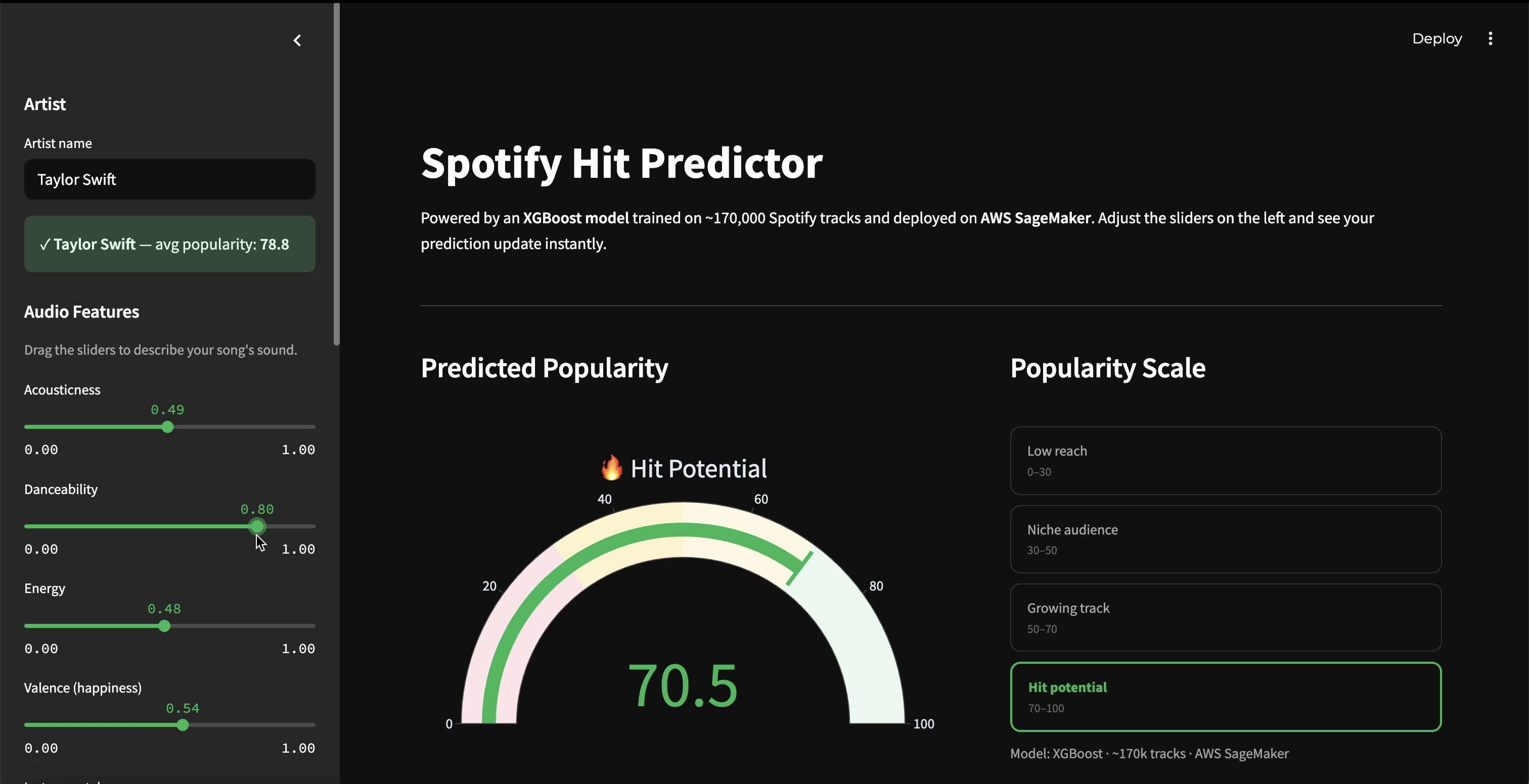
Spotify Hit Predictor app interface

Artist Lookup

Type any artist name,the model retrieves their avg_popularity from training data to anchor the prediction.

Audio Sliders

Adjust danceability, energy, loudness, acousticness, valence, tempo and more in real time.

Instant Prediction

XGBoost model returns a predicted popularity score (0–100) instantly on every input change.

Cloud Deployment

Originally developed on AWS SageMaker. Live demo hosted on Streamlit Community Cloud for persistent public access.

Training Data
Spotify CSV
142,552 tracks
Amazon S3
Train / Validate
/ Test splits
SageMaker Training
XGBoost container
ml.m5.xlarge
SageMaker Endpoint
Real-time inference
 
Streamlit App
Live predictions
Streamlit Cloud
S3 Bucket

Stores train, validate, and test splits. Read directly by SageMaker during training.

Training Job

Spins up a managed instance, trains the model, and saves the artifact back to S3 automatically.

Endpoint

App sends audio features, receives a predicted popularity score (0–100) in milliseconds.

Python 3.11 pandas scikit-learn XGBoost Streamlit Plotly NumPy statsmodels AWS SageMaker Jupyter

Code & Resources

Notebook, Deck & Source

All analysis is fully documented and reproducible. The notebook covers EDA, feature engineering, pre-processing, five model comparisons, hyperparameter tuning, and conclusions in a single file. The presentation deck contains the same findings in slide format.

Jupyter Notebook
Spotify Hit Predictor
Full analysis: EDA, feature engineering, pre-processing pipeline, 5-model comparison, hyperparameter tuning, and conclusions. View on GitHub →
Presentation Deck
Capstone Slide Deck
16-slide PPTX covering dataset, EDA, feature engineering, pre-processing, model comparison, key findings, business implications, and limitations. Download →
GitHub Repository
Full Source Code
Notebooks, Python scripts, Streamlit app code, requirements.txt, and dataset. View on GitHub →
Live Application
Hit Predictor App
Interactive Streamlit app. Enter an artist, set audio feature sliders, get an instant popularity prediction. Launch →